Demo - pyTrigger

Usage example

The purpose of this demo is to show the main functionalities and usages of the trigger python package.

The entire workflow of processing, indeed, is based on the correct usage of the object exposed by the package and called TriggerDB.

First of all, lets start by including the module in our python script as follow:

from trigger import TriggerDB

Now we can create an instance of the object by using a sequential code or a context (recommended).

The second option is recommended since it guarantees the correct logout of the account at the end of the execution.

with TriggerDB() as db:
  print(db)

[INFO] Credentials loaded successfully
<trigger.db.TriggerDB object at 0x78b9280fa2a0>
[INFO] Logout success

As you can notice, an automatic logging of the status of the server is produced, highlighting the correct setup of the account and the final logout.

The db object has a series of private and public member functions: we discourage the usage of the private function unless particular needs.

The entire list of member functions could be listed below:

with TriggerDB() as db:
  print([x for x in dir(db) if not x.startswith('_')])

[INFO] Credentials loaded successfully
['accounts', 'columns', 'from_', 'num_elements', 'select', 'tables']
[INFO] Logout success

Each member function could be used to obtain a different set of information.

The main functionalities for the management of the database tables are described by the following functions:

• tables ➡️ Get the list of available tables

• columns ➡️ Get the list of available columns in the current table

• accounts ➡️ Get the list of available accounts

A common usage of the database, indeed, involves the extraction of records belonging to a particular user account, so, first of all, we need to know the available tables, the set of information stored in that table and the list of possible accounts to check. Lets start by the list of available accounts:

with TriggerDB() as db:
  print(db.accounts())

[INFO] Credentials loaded successfully
[WARN] Maximum limit exceeded. Given 100000 against a maximum of 10000. Automated downgrade to the maximum value
[{'email': 'n.curti1'}, {'email': 'a.merlot'}, {'email': 'cnr00001'}, {'email': 'DE000003'}, {'email': 'CH000004'}, {'email': 'CH000005'}, {'email': 'GR000006'}, {'email': 'GR000007'}, {'email': 'GR000008'}, {'email': 'CH000009'}, {'email': 'DE000010'}, {'email': 'DE000011'}, {'email': 'GR000012'}, {'email': 'DE000013'}, {'email': 'DE000014'}, {'email': 'DE000015'}, {'email': 'GR000016'}, {'email': 'DE000017'}, {'email': 'GR000018'}, {'email': 'DE000019'}, {'email': 'DE000020'}, {'email': 'GR000021'}, {'email': 'DE000022'}, {'email': 'DE000023'}, {'email': 'DE000024'}, {'email': 'GR000025'}, {'email': 'GR000026'}, {'email': 'GR000027'}, {'email': 'GR000028'}, {'email': 'GR000029'}, {'email': 'GR000030'}, {'email': 'GR000031'}, {'email': 'GR000032'}, {'email': 'GR000033'}, {'email': 'GR000034'}, {'email': 'GR000035'}, {'email': 'GR000036'}, {'email': 'GR000037'}, {'email': 'GR000038'}, {'email': 'GR000039'}, {'email': 'GR000040'}, {'email': 'GR000041'}, {'email': 'GR000042'}, {'email': 'GR000043'}, {'email': 'GR000044'}, {'email': 'GR000045'}, {'email': 'GR000046'}, {'email': 'GR000047'}, {'email': 'GR000048'}, {'email': 'GR000049'}, {'email': 'GR000050'}, {'email': 'GR000051'}, {'email': 'GR000052'}, {'email': 'GR000053'}, {'email': 'GR000054'}, {'email': 'GR000055'}, {'email': 'GR000056'}, {'email': 'DE000057'}, {'email': 'IT000058'}, {'email': 'IT000059'}, {'email': 'IT000060'}, {'email': 'IT000061'}, {'email': 'IT000062'}, {'email': 'IT000063'}, {'email': 'IT000064'}, {'email': 'IT000065'}, {'email': 'IT000066'}, {'email': 'GR000067'}, {'email': 'GR000068'}, {'email': 'IT000069'}, {'email': 'GR000070'}, {'email': 'GR000071'}, {'email': 'GR000072'}, {'email': 'GR000073'}, {'email': 'GR000074'}, {'email': 'GR000075'}, {'email': 'DE000076'}, {'email': 'DE000077'}, {'email': 'DE000078'}, {'email': 'DE000079'}, {'email': 'DE000080'}, {'email': 'DE000081'}, {'email': 'DE000082'}, {'email': 'DE000083'}, {'email': 'DE000084'}, {'email': 'DE000085'}, {'email': 'DE000086'}, {'email': 'DE000087'}, {'email': 'DE000088'}, {'email': 'DE000089'}, {'email': 'DE000090'}, {'email': 'DE000091'}, {'email': 'IT000092'}, {'email': 'GR000093'}, {'email': 'GR000094'}, {'email': 'GR000095'}, {'email': 'GR000096'}, {'email': 'GR000097'}, {'email': 'GR000098'}, {'email': 'GR000099'}, {'email': 'GR000100'}, {'email': 'm.carell'}, {'email': 'i.diembe'}, {'email': 's.disaba'}, {'email': 'e.bratti'}, {'email': 'a.hoffma'}, {'email': 'c.perdik'}, {'email': 'a.spadot'}, {'email': 'CH000108'}, {'email': 'IT000109'}, {'email': 'IT000110'}, {'email': 'GR000111'}, {'email': 'GR000112'}, {'email': 'CH000113'}, {'email': 'CH000114'}, {'email': 'CH000115'}, {'email': 'CH000116'}, {'email': 'CH000117'}, {'email': 'CH000118'}, {'email': 'DE000119'}, {'email': 'DE000120'}, {'email': 'DE000121'}, {'email': 'DE000122'}, {'email': 'DE000123'}, {'email': 'DE000124'}, {'email': 'DE000125'}, {'email': 'CH000126'}, {'email': 'CH000127'}, {'email': 'CH000128'}, {'email': 'GR000129'}, {'email': 'CH000130'}, {'email': 'IT000131'}, {'email': 'CH000132'}, {'email': 'IT000133'}, {'email': 'GR000134'}, {'email': 'GR000135'}, {'email': 'GR000136'}, {'email': 'GR000137'}, {'email': 'IT000138'}, {'email': 'IT000139'}, {'email': 'GR000140'}, {'email': 'a.fuschi'}, {'email': 'GR000142'}, {'email': 'IT000143'}, {'email': 'GR000144'}]
[INFO] Logout success

This is out first query on the database and you can notice that the output is a standard JSON made by a list of dictionaries.

To facilitate the readability of the output we can use the pandas package to convert it into a dataframe as follow:

import pandas as pd

with TriggerDB() as db:
  df = pd.json_normalize(db.accounts())

df

[INFO] Credentials loaded successfully
[WARN] Maximum limit exceeded. Given 100000 against a maximum of 10000. Automated downgrade to the maximum value
[INFO] Logout success

	email
0	n.curti1
1	a.merlot
2	cnr00001
3	DE000003
4	CH000004
...	...
140	GR000140
141	a.fuschi
142	GR000142
143	IT000143
144	GR000144

145 rows × 1 columns

In this way we can easily manipulate the amount of information get by the query and see the amount of accounts registered in the current database.

The next processing involves the available tables and information stored in them.

To this purpose we can use the combination of tables and columns member functions as follow:

with TriggerDB() as db:
  tables = db.tables()
  print(f'Available tables: {tables}')
  for tab in tables:
    print(f'  {tab}: {db.columns(tab)}')

[INFO] Credentials loaded successfully
Available tables: ['myair', 'ecg', 'ppg', 'gps', 'sleep', 'smartwatchlow', 'smartwatchhigh', 'accounts']
  myair: ['email', 'userId', 'year', 'month', 'day', 'hour', 'minute', 'second', 'pm1', 'pm25', 'pm10', 'pc03', 'pc05', 'pc1', 'pc25', 'pc5', 'pc10', 'temperature', 'humidity', 'pressure', 'sound', 'uvb', 'light']
  ecg: ['email', 'userId', 'year', 'month', 'day', 'hour', 'minute', 'second', 'microsecond', 'ecg']
  ppg: ['email', 'userId', 'year', 'month', 'day', 'hour', 'minute', 'second', 'microsecond', 'ppg']
  gps: ['email', 'userId', 'year', 'month', 'day', 'hour', 'minute', 'second', 'longitude', 'latitude', 'accuracy']
  sleep: ['email', 'userId', 'year', 'month', 'day', 'hour', 'minute', 'second', 'sleepduration', 'awake', 'insomnia', 'remsleep', 'lightsleep', 'deepsleep', 'sleepquality']
  smartwatchlow: ['email', 'userId', 'year', 'month', 'day', 'hour', 'minute', 'second', 'step', 'cal', 'bphigh', 'bplow', 'bodytemp']
  smartwatchhigh: ['email', 'userId', 'year', 'month', 'day', 'hour', 'minute', 'second', 'heartrate', 'sleeprate', 'oxygens']
  accounts: ['id', 'email', 'created_at', 'last_login']
[INFO] Logout success

From this overview we can notice that each column has always an email column which lists the information get by our previous analysis about the amount of accounts. The email information represents the link between the users and the information stored into the several tables and it could be used to extract the data associated to each account.

Starting from these information, we are now ready to perform our first (realistic) query on the database.

To this purpose, the trigger package provides two different interface: standard and chaining.

For a better readability of the code and a correct management of the desired query, we encourage the use of the chaining modality: for sake of completeness, the standard way can be easily addressed by calling the select member function of the object.

The chaining modality could be used by calling the from_ member function which requires the table that we want to analyze.

with TriggerDB() as db:
  res = (
    db.from_('myair')
      .select('email', 'year', 'month', 'day', 'hour', 'minute', 'second', 'temperature', 'humidity', 'pressure')
      .where(year='=2025', month='=9', day='=10', hour='>=0', email='=DE000086')
      .order_by('second')
      .asc()
      .limit(10000)
      .fetch()
  )

df = pd.json_normalize(res)
df

[INFO] Credentials loaded successfully
[INFO] Logout success

	email	year	month	day	hour	minute	second	temperature	humidity	pressure
0	DE000086	2025	9	10	9	56	4	27	78	1015
1	DE000086	2025	9	10	10	0	4	28	60	1013
2	DE000086	2025	9	10	10	4	4	28	80	1013
3	DE000086	2025	9	10	10	8	4	29	54	991
4	DE000086	2025	9	10	10	12	4	28	52	965
...	...	...	...	...	...	...	...	...	...	...
340	DE000086	2025	9	10	11	58	4	27	78	1012
341	DE000086	2025	9	10	12	2	4	29	77	1012
342	DE000086	2025	9	10	12	6	4	30	76	1012
343	DE000086	2025	9	10	12	10	4	31	74	1012
344	DE000086	2025	9	10	12	14	4	31	72	1012

345 rows × 10 columns

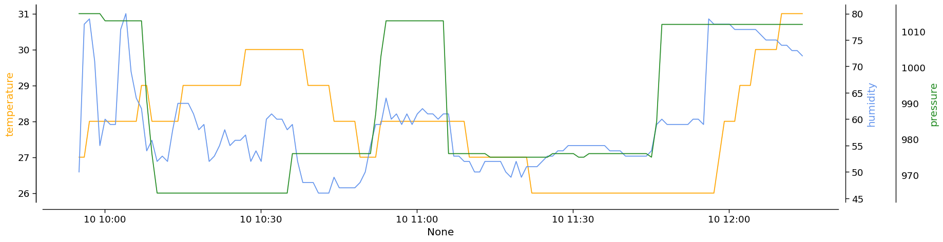
Now we can easily display the trend of the climate variables for the selected day:

import pylab as plt
import seaborn as sns

time = pd.to_datetime(df[['year', 'month', 'day', 'hour', 'minute', 'second']], format='%Y-%m-%d %H:%M:%S.%f')

with sns.plotting_context('paper', font_scale=1.5):
  fig, ax = plt.subplots(nrows=1, ncols=1, figsize=(20, 5))
  sns.lineplot(
    ax=ax,
    x=time,
    y=df['temperature'],
    color='orange',
  )
  ax1 = ax.twinx()
  sns.lineplot(
    ax=ax1,
    x=time,
    y=df['humidity'],
    color='cornflowerblue',
  )
  ax2 = ax.twinx()
  sns.lineplot(
    ax=ax2,
    x=time,
    y=df['pressure'],
    color='forestgreen',
  )
  sns.despine(
    ax=ax,
    top=True,
    right=True,
    left=False,
    bottom=False,
    offset=10
  )
  sns.despine(
    ax=ax1,
    top=True,
    right=False,
    left=False,
    bottom=True,
    offset=10
  )

  sns.despine(
    ax=ax2,
    top=True,
    right=False,
    left=True,
    bottom=True,
    offset=80
  )

  ax.set_ylabel('temperature', color='orange')
  ax1.set_ylabel('humidity', color='cornflowerblue')
  ax2.set_ylabel('pressure', color='forestgreen')